scipy.stats.skellam

scipy.stats.skellam = <scipy.stats._discrete_distns.skellam_gen object at 0x2aba95116310>

A Skellam discrete random variable.

As an instance of the rv_discrete class, skellam object inherits from it a collection of generic methods (see below for the full list), and completes them with details specific for this particular distribution.

Notes

Probability distribution of the difference of two correlated or uncorrelated Poisson random variables.

Let k1 and k2 be two Poisson-distributed r.v. with expected values lam1 and lam2. Then, k1 - k2 follows a Skellam distribution with parameters mu1 = lam1 - rho*sqrt(lam1*lam2) and mu2 = lam2 - rho*sqrt(lam1*lam2), where rho is the correlation coefficient between k1 and k2. If the two Poisson-distributed r.v. are independent then rho = 0.

Parameters mu1 and mu2 must be strictly positive.

For details see: http://en.wikipedia.org/wiki/Skellam_distribution

skellam takes mu1 and mu2 as shape parameters.

The probability mass function above is defined in the “standardized” form. To shift distribution use the loc parameter. Specifically, skellam.pmf(k, mu1, mu2, loc) is identically equivalent to skellam.pmf(k - loc, mu1, mu2).

Examples

>>> from scipy.stats import skellam
>>> import matplotlib.pyplot as plt
>>> fig, ax = plt.subplots(1, 1)

Calculate a few first moments:

>>> mu1, mu2 = 15, 8
>>> mean, var, skew, kurt = skellam.stats(mu1, mu2, moments='mvsk')

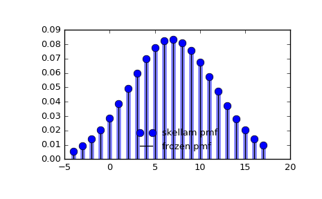
Display the probability mass function (pmf):

>>> x = np.arange(skellam.ppf(0.01, mu1, mu2),
...               skellam.ppf(0.99, mu1, mu2))
>>> ax.plot(x, skellam.pmf(x, mu1, mu2), 'bo', ms=8, label='skellam pmf')
>>> ax.vlines(x, 0, skellam.pmf(x, mu1, mu2), colors='b', lw=5, alpha=0.5)

Alternatively, the distribution object can be called (as a function) to fix the shape and location. This returns a “frozen” RV object holding the given parameters fixed.

Freeze the distribution and display the frozen pmf:

>>> rv = skellam(mu1, mu2)
>>> ax.vlines(x, 0, rv.pmf(x), colors='k', linestyles='-', lw=1,
...         label='frozen pmf')
>>> ax.legend(loc='best', frameon=False)
>>> plt.show()

(Source code)

Check accuracy of cdf and ppf:

>>> prob = skellam.cdf(x, mu1, mu2)
>>> np.allclose(x, skellam.ppf(prob, mu1, mu2))
True

Generate random numbers:

>>> r = skellam.rvs(mu1, mu2, size=1000)

Methods

rvs(mu1, mu2, loc=0, size=1, random_state=None)	Random variates.
pmf(x, mu1, mu2, loc=0)	Probability mass function.
logpmf(x, mu1, mu2, loc=0)	Log of the probability mass function.
cdf(x, mu1, mu2, loc=0)	Cumulative distribution function.
logcdf(x, mu1, mu2, loc=0)	Log of the cumulative distribution function.
sf(x, mu1, mu2, loc=0)	Survival function (also defined as 1 - cdf, but sf is sometimes more accurate).
logsf(x, mu1, mu2, loc=0)	Log of the survival function.
ppf(q, mu1, mu2, loc=0)	Percent point function (inverse of cdf — percentiles).
isf(q, mu1, mu2, loc=0)	Inverse survival function (inverse of sf).
stats(mu1, mu2, loc=0, moments='mv')	Mean(‘m’), variance(‘v’), skew(‘s’), and/or kurtosis(‘k’).
entropy(mu1, mu2, loc=0)	(Differential) entropy of the RV.
expect(func, args=(mu1, mu2), loc=0, lb=None, ub=None, conditional=False)	Expected value of a function (of one argument) with respect to the distribution.
median(mu1, mu2, loc=0)	Median of the distribution.
mean(mu1, mu2, loc=0)	Mean of the distribution.
var(mu1, mu2, loc=0)	Variance of the distribution.
std(mu1, mu2, loc=0)	Standard deviation of the distribution.
interval(alpha, mu1, mu2, loc=0)	Endpoints of the range that contains alpha percent of the distribution