scipy.stats.multivariate_normal

scipy.stats.multivariate_normal = <scipy.stats._multivariate.multivariate_normal_gen object at 0x2aba953e48d0>

A multivariate normal random variable.

The mean keyword specifies the mean. The cov keyword specifies the covariance matrix.

Parameters:

x : array_like

Quantiles, with the last axis of x denoting the components.

mean : array_like, optional

Mean of the distribution (default zero)

cov : array_like, optional

Covariance matrix of the distribution (default one)

allow_singular : bool, optional

Whether to allow a singular covariance matrix. (Default: False)

random_state : None or int or np.random.RandomState instance, optional

If int or RandomState, use it for drawing the random variates. If None (or np.random), the global np.random state is used. Default is None.

Alternatively, the object may be called (as a function) to fix the mean

and covariance parameters, returning a “frozen” multivariate normal

random variable:

rv = multivariate_normal(mean=None, cov=1, allow_singular=False)

• Frozen object with the same methods but holding the given mean and covariance fixed.

Notes

Setting the parameter mean to None is equivalent to having mean

be the zero-vector. The parameter cov can be a scalar, in which case the covariance matrix is the identity times that value, a vector of diagonal entries for the covariance matrix, or a two-dimensional array_like.

The covariance matrix cov must be a (symmetric) positive semi-definite matrix. The determinant and inverse of cov are computed as the pseudo-determinant and pseudo-inverse, respectively, so that cov does not need to have full rank.

The probability density function for multivariate_normal is

\[f(x) = \frac{1}{\sqrt{(2 \pi)^k \det \Sigma}} \exp\left( -\frac{1}{2} (x - \mu)^T \Sigma^{-1} (x - \mu) \right),\]

where \(\mu\) is the mean, \(\Sigma\) the covariance matrix, and \(k\) is the dimension of the space where \(x\) takes values.

New in version 0.14.0.

Examples

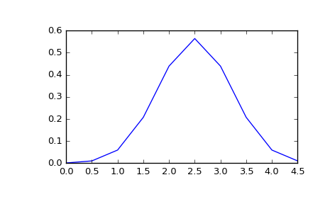
>>> import matplotlib.pyplot as plt
>>> from scipy.stats import multivariate_normal

>>> x = np.linspace(0, 5, 10, endpoint=False)
>>> y = multivariate_normal.pdf(x, mean=2.5, cov=0.5); y
array([ 0.00108914,  0.01033349,  0.05946514,  0.20755375,  0.43939129,
        0.56418958,  0.43939129,  0.20755375,  0.05946514,  0.01033349])
>>> fig1 = plt.figure()
>>> ax = fig1.add_subplot(111)
>>> ax.plot(x, y)

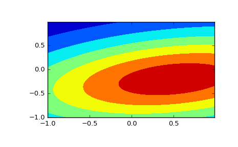
The input quantiles can be any shape of array, as long as the last axis labels the components. This allows us for instance to display the frozen pdf for a non-isotropic random variable in 2D as follows:

>>> x, y = np.mgrid[-1:1:.01, -1:1:.01]
>>> pos = np.dstack((x, y))
>>> rv = multivariate_normal([0.5, -0.2], [[2.0, 0.3], [0.3, 0.5]])
>>> fig2 = plt.figure()
>>> ax2 = fig2.add_subplot(111)
>>> ax2.contourf(x, y, rv.pdf(pos))

(Source code)

Methods

pdf(x, mean=None, cov=1, allow_singular=False)	Probability density function.
logpdf(x, mean=None, cov=1, allow_singular=False)	Log of the probability density function.
rvs(mean=None, cov=1, size=1, random_state=None)	Draw random samples from a multivariate normal distribution.
entropy()	Compute the differential entropy of the multivariate normal.