scipy.signal.freqz
- scipy.signal.freqz(b, a=1, worN=None, whole=False, plot=None)[source]
Compute the frequency response of a digital filter.
Given the M-order numerator b and N-order denominator a of a digital filter, compute its frequency response:
            jw               -jw               -jwM
   jw    B(e  )  b[0] + b[1]e    + .... + b[M]e
H(e  ) = ---- = -----------------------------------
            jw               -jw               -jwN
         A(e  )  a[0] + a[1]e    + .... + a[N]e
Parameters: b : array_like
numerator of a linear filter
a : array_like
denominator of a linear filter
worN : {None, int, array_like}, optional
If None (default), then compute at 512 frequencies equally spaced around the unit circle. If a single integer, then compute at that many frequencies. If an array_like, compute the response at the frequencies given (in radians/sample).
whole : bool, optional
Normally, frequencies are computed from 0 to the Nyquist frequency, pi radians/sample (upper-half of unit-circle). If whole is True, compute frequencies from 0 to 2*pi radians/sample.
plot : callable
A callable that takes two arguments. If given, the return parameters w and h are passed to plot. Useful for plotting the frequency response inside freqz.
Returns: w : ndarray
The normalized frequencies at which h was computed, in radians/sample.
h : ndarray
The frequency response.
Notes
Using Matplotlib’s “plot” function as the callable for plot produces unexpected results, this plots the real part of the complex transfer function, not the magnitude. Try lambda w, h: plot(w, abs(h)).
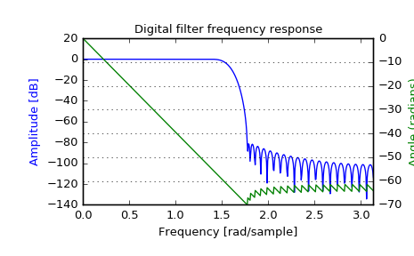
Examples
>>> from scipy import signal
>>> b = signal.firwin(80, 0.5, window=('kaiser', 8))
>>> w, h = signal.freqz(b)
>>> import matplotlib.pyplot as plt
>>> fig = plt.figure()
>>> plt.title('Digital filter frequency response')
>>> ax1 = fig.add_subplot(111)
>>> plt.plot(w, 20 * np.log10(abs(h)), 'b')
>>> plt.ylabel('Amplitude [dB]', color='b')
>>> plt.xlabel('Frequency [rad/sample]')
>>> ax2 = ax1.twinx()
>>> angles = np.unwrap(np.angle(h))
>>> plt.plot(w, angles, 'g')
>>> plt.ylabel('Angle (radians)', color='g')
>>> plt.grid()
>>> plt.axis('tight')
>>> plt.show()