scipy.signal.convolve

scipy.signal.convolve(in1, in2, mode='full')

Convolve two N-dimensional arrays.

Convolve in1 and in2, with the output size determined by the mode argument.

Parameters:

in1 : array_like

First input.

in2 : array_like

Second input. Should have the same number of dimensions as in1. If operating in ‘valid’ mode, either in1 or in2 must be at least as large as the other in every dimension.

mode : str {‘full’, ‘valid’, ‘same’}, optional

A string indicating the size of the output:

full

The output is the full discrete linear convolution of the inputs. (Default)

valid

The output consists only of those elements that do not rely on the zero-padding.

same

The output is the same size as in1, centered with respect to the ‘full’ output.

Returns:

convolve : array

An N-dimensional array containing a subset of the discrete linear convolution of in1 with in2.

See also

numpy.polymul

performs polynomial multiplication (same operation, but also accepts poly1d objects)

Examples

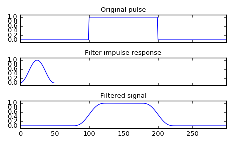
Smooth a square pulse using a Hann window:

>>> from scipy import signal
>>> sig = np.repeat([0., 1., 0.], 100)
>>> win = signal.hann(50)
>>> filtered = signal.convolve(sig, win, mode='same') / sum(win)

>>> import matplotlib.pyplot as plt
>>> fig, (ax_orig, ax_win, ax_filt) = plt.subplots(3, 1, sharex=True)
>>> ax_orig.plot(sig)
>>> ax_orig.set_title('Original pulse')
>>> ax_orig.margins(0, 0.1)
>>> ax_win.plot(win)
>>> ax_win.set_title('Filter impulse response')
>>> ax_win.margins(0, 0.1)
>>> ax_filt.plot(filtered)
>>> ax_filt.set_title('Filtered signal')
>>> ax_filt.margins(0, 0.1)
>>> fig.tight_layout()
>>> fig.show()

(Source code)